One popular argument we often hear from investors that I speak with as part of my work at Mutiny Funds is “I’m a long-term investor. Short-term volatility or drawdowns don’t matter to us because I am happy to hold the assets for the long-term.”
I hear this particularly from people who have learned about investing a lot from the Warren Buffett/Jack Bogle camp as they often are quoted in soundbites to this effect. (though, I think their actual views are significantly more nuanced and sophisticated than the naive interpretation of that statement).
Benn Eifert, CIO of QVR, noted and articulated that these sorts of statements often belie a misunderstanding of how compound growth actually works and I’d like to explore that a bit.
Here’s a trivia question: You have two return streams (e.g., two stocks or two trading strategies). You know that both will average1 an annual return of 10%.2
There is only one difference between the two return streams:
- The first return stream, let’s call it Valley Path, has an annualized volatility of 10%.3 Like walking through a valley with rolling hills, it’s just modestly chugging along.
- The second return stream, let’s call it Mountain Climb, has an annualized volatility of 20%. It’s scaling up and down a series of steep mountains.
In investing terms, which one will have a higher compounded annual growth rate or will they be the same? (don’t look down the page and cheat!)
- Valley Path (10% annual return/10% volatility) will have a higher compounded annual growth rate
- Mountain Climb (10% annual return/20% volatility) will have a higher compounded annual growth rate
- They will have the same compounded annual growth rate.
Got your answer?
The long-term compound growth rate for taking the Valley Path return stream will be 9.5%, while the long-term compounded growth rate for taking the Mountain Climb will be 8%.
How can two return streams with the same average annual returns have different compounded growth rates?
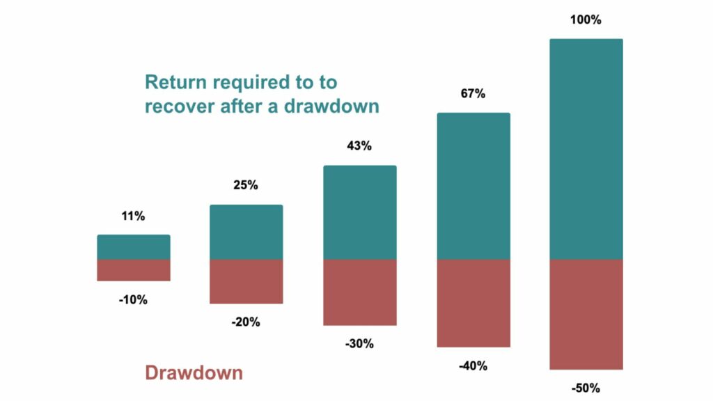
As a simple example, let’s say you have a $1 million portfolio. In Year 1, it suffers a 50% drawdown. Ouch!
The next year ends with a breathtaking rally of 100%. Amazing!
Over that two-year period, your average annual return is a positive 25%.4

However, what is the total portfolio value at the end of the second year? Well, your $1 million declined to $500,000 in Year 1 (a loss of -50%) and then grew 100% from there to get back to exactly where you started: $1 million, a 0% compounded growth rate.
If your goal is to grow your wealth over time, the compounded growth rate is all that matters. Having a big boom followed by big bust years drags down the rate of compounding compared to a ‘smoother’ path.
Despite the breathtaking rally, your wealth is not growing over that time period, merely recovering to where it started.
All else equal – the more volatility in a return stream, the worse the long-term returns.
A 10% average annual return stream with 40% volatility will compound at only 2% per year.
A 10% average annual return stream with 50% volatility will actually lose money over time!
In our hiking analogy, you’re spending energy going vertically up and down the mountain (volatility) instead of using that same energy to move ‘horizontally’ across the terrain (compound growth).
The Northwest face of Half Dome in Yosemite national park is a famous big-wall climbing route. It’s about 2,200 feet high and is one of the original technical climbing routes up Half Dome. This climb is typically rated 5.12 or 5.13 which is considered a very difficult climb requiring advanced rock climbing skills.
For an experienced and well-prepared climbing team, it often takes between two and three days to complete the route. Rock climbing burns around 700 calories per hour. Assuming 8 hours per day of climbing over three days, it will require 16,800 calories to get to the top.

The Eastern side can be climbed by a hiker without any climbing skills. It’s still a pretty strenuous hike of about 15 miles round trip with an elevation gain of 4,800 feet. That’s no joke, but it’s doable in about 12 hours by a reasonably fit individual. Hiking burns around 500 calories per hour so a 12 hour hike would require about 6,000 calories.
Whichever route you take, you end up in the same place but the climb requires double the time and energy. While I can admire the climber with the skill and fitness to take the harder route in the case of Half Dome, I’m not trying to make my investing journey three times harder or longer.
Compare the investor who had -50% loss followed by the big 100% rally to get back to even versus an investor who had the same average return of 25% over two years but rather than big wins and big losses. In this example, their portfolios grows exactly 25% in year one and 25% in year two. The second investor, with just no volatility in the return stream, ends the two year period with $1,562,500, a gain of 56.2%.
Play this out further and we can see that two portfolios with the same average returns can have wildly different growth rates.
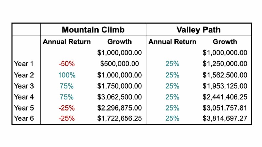
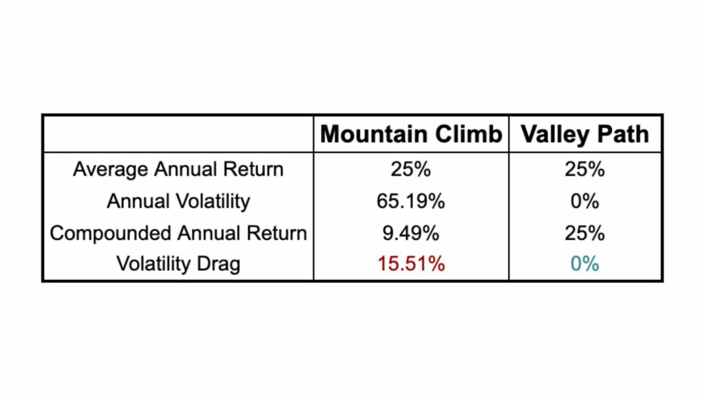
Even though both these two portfolios have an average annual return of 25%, their long-term growth rate is very different.
This is the Iron Law of Volatility Drag: the higher the volatility of a portfolio, the worse the long-term compound rate of growth of a portfolio (all else being equal).5
Reducing the volatility of a return stream also helps to address the second part of our Dual Mandate: Don’t Die Tryin’
The investor that gets exactly a 25% return per year doesn’t have the same sequencing risk that the investor who gets either 100% or -50% returns.
As with Nick and Nancy, if the investor on the Mountain Climb needs to withdraw funds the year they are down 50% because of unplanned illness, college tuition, or a leaky roof – their returns can be even worse.
Let’s say the Mountain Climb investors need to withdraw $50,000 from their portfolio after year 1 due to an unplanned emergency. Their $500,000 drops to $450,000. The breathtaking rally now and their wealth doubles to $900,000. Due to the unplanned withdrawal, their wealth after year 2 has declined by $100,000 compared to the scenario without the withdrawal.
Lest this seem a little too tin foil hat, it’s not as unusual as many people. As mathematician Benoit Mandelbrot noted in the 1960s – volatility clusters.6 In the more memorable words of Vladimir Lenin:
“There are decades where nothing happens; and there are weeks where decades happen.”
In 2008, many people discovered the stock market declined, their home values declined, and incomes fell. Just when people most needed their savings most was the worst time to withdraw them. In 2022, many tech workers that had all their savings invested in the Nasdaq found out that their incomes and tech stocks were more correlated than they had expected.
As an individual, the average returns of the market are not what matters to you. What matters is your returns.
If you had to withdraw money from your investment accounts in 2009 to make ends meet while you looked for a new job or your business faltered, you would be better off with a portfolio closer to the Valley Path.
To reduce drawdowns and more effectively compound wealth over the long term requires true diversification. I believe the easiest way to think about this is as categorizing assets as either offensive (risk-on) or defensive (risk-off).
The offensive bucket is most easily thought of as any long GDP asset, typically correlated to the S&P 500 and broad economic growth. These include: stocks, bonds, private equity, venture capital, and real estate. They are assets that perform well most of the time, but when they perform badly, they perform really badly as we’ve seen in prior crises such as 2008 or 2001.
In the defensive bucket would be anything that is short GDP, typically uncorrelated or negatively correlated to the S&P 500. Defensive assets include things like commodities, Gold, and long volatility/tail risk option strategies. They are assets that can struggle for longer periods of time, but they perform well at the time when the offense needs it the most, providing effective diversification across decades of market cycles.
Many of the same investors that say they don’t care about short-term volatility or drawdowns think that they are smarter in the long run: “I don’t want to invest in defensive assets because I am a long-term investor and defensive assets have poor long-term returns. I care about the long-term returns and I can tolerate the drawdowns.”
The Iron Law of Volatility Drag shows you need both offense and defense to minimize the volatility of the portfolio, but also to get the best long-term returns.
Let’s look at what happens when you add a little defense to an offense-only investment strategy.
For this example, consider a simple defensive strategy, buying put options on the S&P.7
If you’re familiar with options trading, skip down to the chart below, if not here’s a quick explanation:
An option is a financial instrument that allows investors to buy and sell the right, but not the obligation (i.e. the “option”) to buy or sell an underlying asset at a specified time at a specified price.
- Call options allow the holder to buy the asset at a specified time at a specified price. A call option generally benefits when the price of the underlying asset increases over time so it is a bet on the market going up.
- Put options allow the holder to sell the asset at a specified time at a specified price. A put option generally benefits if the price of the underlying asset will decrease so it is a bet on the market going down.
For example, if there is a stock currently trading at $100, you could buy a put option for the right to sell the asset at a specified time (say the end of next month) at a specified strike price (say $90).
Let’s say this option costs $1. So, you pay $1 up front for the right to sell the stock for $90 at the end of the coming month. If the price of the stock falls to $85 in that time period, you can buy the stock for $85 in the market and use your option contract to sell it for $90. Once you deduct the $1 you paid for the option, you pocket a $4 profit .
If the stock ends the month at any price higher than $90, then the option expires worthless and you lose the $1 you paid for the option.
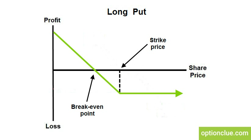
In this example, your maximum potential loss over this time period is $11, the cost you paid for the option plus the $10 difference between the current price and the strike price of the option you bought.
A put option is conceptually similar to an insurance policy. When you buy health insurance, typically you pay the premium up front (~= the price of the option) then you are on the hook for the deductible (the difference between the strike price and current price). Beyond that, the insurance kicks in and covers any expenses. If you have a $5,000 premium and $10,000 deductible in a calendar year then your maximum loss is capped at $15,000 for that year. Even if you get hit by a bus and rack up a million dollars in medical bills, you’re only on the hook for $15,000.8
The price of the option (in this case, $1) is equivalent to an insurance premium that you pay whether you use the insurance or not. If you own one share of the stock at $100 and you pay $1 for the put option with a $90 strike price then the $10 difference between the current price and the strike price is similar to your deductible. You can lose $10 “out of pocket” before the insurance kicks in. Buying this put option costs you something ($1), but you are guaranteeing that you can’t lose more than $11 over that time period, effectively capping your losses similar to how most insurance policies work.
Similar to buying insurance, put buying by itself is a long-term losing strategy. Over the long run, insurance companies are profitable so the total premiums paid in is more than the amount paid out. On average, policyholders lose. However, this doesn’t mean buying insurance is dumb!
As expected, the performance of our put buying strategy on the S&P doesn’t look very attractive. Over a nearly 20 year period, it has lost money.
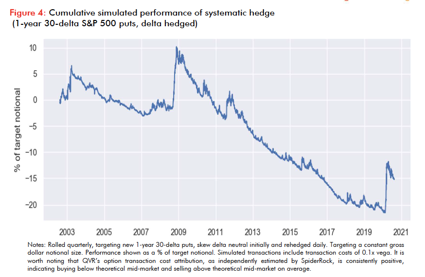
Why would anyone invest in this defensive strategy that loses money over time when they could invest in something that makes money over time?
The popular understanding I most often hear is that it’s because these people are “scared” or “not thinking long-term.”
Eifert did some research adding this exact (money-losing) strategy to a 60% stock/40% bond portfolio with quarterly rebalancing between all three components.
The blue line is the 60% stock/40% bond portfolio and the orange line includes adding in the put buying strategy.
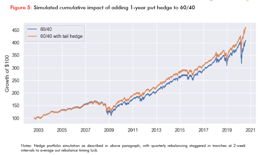
The portfolio which includes the money-losing defensive strategy has higher long-term returns.
How can adding a strategy which loses money over the long-term increase the portfolio returns? Because of the Iron Law of Volatility Drag.
Even though the defensive strategy loses money on average, it makes money at the times when the rest of the portfolio struggles. The outsized performance of the defensive during large market drawdowns allows a regularly rebalanced portfolio to buy risky assets in the periods immediately following those large market drawdowns.
It reduces the total volatility of the portfolio enough to compensate for the fact that it is a losing strategy as a stand-alone.
That’s why effective diversification including both offensive and defensive strategies can make such a big impact on long-term wealth.
I believe that the best portfolios are equal parts offense and defense. Defensive strategies like the put buying strategy tend to look worse as a standalone and so investors fail to incorporate them in their portfolios, even though they improve the overall performance of the portfolio.
By including equal parts offense and defense, an investor seeks to achieve the “free lunch” of diversification:
- They are seeking to maximize terminal wealth…
- while also minimizing drawdowns so that you can have confidence that their savings will be there when you need it.
Though these are the goals that most investors have for their wealth, few investors actually structure their portfolios to achieve them.
If your goal is to maximize your expected long-term wealth while also knowing you’ll be able to handle whatever life comes at you, you need both offensive and defensive assets in your portfolio.
H/t and Image Credits to Benn Eifert.
Footnotes
- For the more mathematically inclined reader, please note that “average” as used throughout this paper refers to the arithmetic mean where compound annual growth rate (CAGR) refers to the geometric mean. We use them in this way as this is how they are typically used in financial publications and research in our experience.
- As will become very apparent if it is not already, we believe it’s impossible to know what some asset will return in the future but bear with me for this stylized example.
- Annualized volatility refers to the standard deviation of an investment’s returns over a one-year period. Saying a Return Stream has an annualized Volatility of 10% means that, assuming the data distribution is approximately normal, about 68 percent of the years there will be a 10% or less move in the price. In the real world of investing, distributions are, in fact, not normal. But for the purposes of this example, that’s not super relevant and the important thing is just to note that one of these investments is more volatile than the other.
- As mentioned in a prior footnote, this is the difference between arithmetic averages and geometric averages. A lot of financial media quotes arithmetic averages (25% in that case), but what matters to long term wealth is the geometric average (0% in this case).
- As with any time that someone uses the phrase “all else equal” – all else is not equal outside this stylized example. I’ll return to that and address it shortly. However, I think it’s important to understand the concept of volatility drag in principle before we make it any more complicated.
- https://en.wikipedia.org/wiki/Volatility_clustering
- This example will use 1-year 30-delta puts, delta hedged and rolled quarterly.
- There are, of course, a gajillion clauses in practice that insurance companies use to try and avoid paying out claims, so this is simplified, but you get the point.
