Sequencing Risk: Why The Expected Value Is Not What You Should Expect
Expected value (EV) is a popular and often cited concept among investors. However, it’s a bit of a misnomer and has a few serious limitations.
To briefly recap, expected value is a calculation made by multiplying the probability of something happening by the magnitude of the outcome.
Let’s say you give me a bet on a fair die. The die has 6 sides so each side should show up 16.6% of the time – that’s 6 to 1 odds.
Now let’s say I offer you a bet that gives you 10 to 1 odds. You bet $1. If you are right, you win $10. If you are wrong, you lose $1.
Would you take this bet?
It probably won’t be the number you guess so you’ll probably lose a dollar. However, the concept of expected value suggests this is a good bet.
The probability of the die coming up on the number you guess is 16.6% and you get 10 to 1 odds. To calculate the expected value, you multiply the probability * magnitude of your winnings.
In this case, the expected value of your $1 bet is $1.66. You have a 16.6% of being right multiplied by a $10 payoff (16.6% * $10 = $1.66).
This is an attractive bet: You are risking $1 and your expected payoff is $1.66.
Expected value is an important concept to understand that has broad applications across your life. Whether you are making an investment, career decision, or business decision, expected value is a valuable and important lens for thinking about it. 1
In my experience, the vast majority of investors use expected value as the primary model for thinking about an investment. When evaluating a new investment opportunity, they tend to try and determine the expected value of an investment and how it compares with other things they could invest in and to invest in the things which seem to have the highest expected value.
Most investing discussions are discussions around the EV (or risk-adjusted EV2
) of different assets or strategies.
Generally, a good understanding of expected value and some common sense will get you pretty far, but it’s important to understand the limitations of thinking strictly in these terms. I call these the Four Horsemen of Expected Value.
Consider the following thought experiment:3
In scenario one, which we will call the ensemble scenario, one hundred different people go to Caesar’s Palace Casino to gamble. Each brings $1,000 and has a few rounds of gin and tonic on the house. Some will lose, some will win and we can infer at the end of the day what the “edge” is.
Let’s say in this example that our gamblers are all very smart (or cheating). They are using a particular strategy which, on average, makes a 50% return each day.
However, this strategy also has the risk that, on average, one gambler out of the 100 loses all their money and goes bust. In this case, let’s say gambler number 28 blows up. Will gambler number 29 be affected? Not in this example. The outcomes of each individual gambler are separate and don’t depend on how the other gamblers fare.
You can calculate that, on average, each gambler makes about $500 per day and about 1% of the gamblers will go bust every day. Using a standard expected value analysis, you have a 99% chance of gains and an expected average return of 50%.
You are risking $1000 and your expected value of playing is $1495.
Seems like a pretty sweet deal right?
Now compare this to scenario two, the path scenario. In this scenario, one person – Theodorus, goes to Caesar’s Palace a hundred days in a row, starting with $1,000 on day one and employing the same strategy. He makes 50% on day 1 and so goes back on day 2 with $1,500. He makes 50% again and goes back on day 3 and makes 50% again, now sitting at $3,375. On Day 18, he has turned his $1,000 into $1 million. On day 27, Theodorus has $56 million and is walking out of Caesar’s on a cloud.
But, when day 28 strikes, cousin Theodorus goes bust. He loses everything. Will there be a day 29? Nope, he’s broke and there is nothing left to gamble with.
The probabilities of success from the collection of people do not apply to one person. You can safely calculate that by using this strategy, Theodorus has a 100% probability of eventually going bust. Though a standard expected value analysis would suggest this is a good strategy, it is actually a very bad strategy for a single person to pursue over time.
The first scenario is an example of ensemble probability and the second one is an example of what we can call path probability. The first is concerned with a collection of people and the other with a single person through time.
In an ensemble probability, the ruin of one individual does not affect the others. In a time probability, the ruin at one point in time affects all future points in time.
This thought experiment is an example of ergodicity. Any actor taking part in a system can be defined as either ergodic or non-ergodic.
What is Ergodicity?
In an ergodic scenario, the average outcome of the group is the same as the average outcome of the individual over time. An example of an ergodic system would be the outcomes of a coin toss (heads/tails). If 100 people flip a coin once or 1 person flips a coin 100 times, you get the same distribution of outcomes.
A more fun (or perhaps more morbid) example is Russian Roulette. Take a game of Russian Roulette as an example. If you survive, you win $1,000,000.
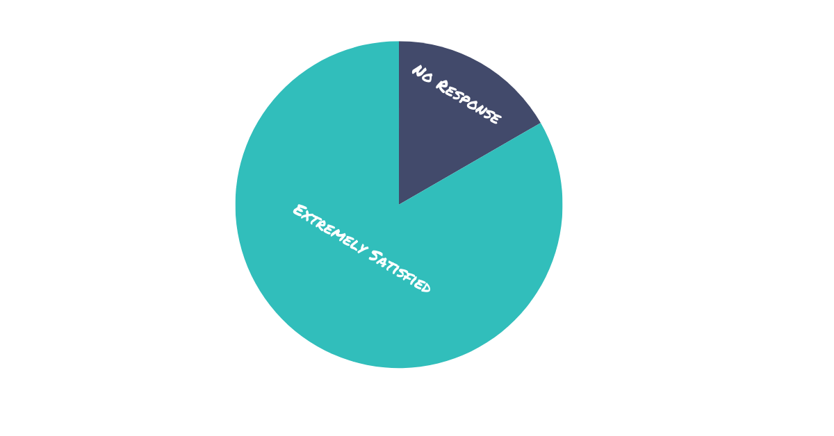
If 6 different players play Russian Roulette and you conducted an after that fact survey, 5 out of every 6 Russian roulette players would recommend it as a very exciting and profitable game.
Post-purchase survey for a single game of Russian Roulette.
You might roll the dice and take $1,000,000 to play Russian Roulette one time (though I wouldn’t advise it!). But there’s no amount of money that would make you play it 6 times in a row. You are guaranteed to lose!
Russian Roulette is non-ergodic – you don’t get the same outcome of 6 people playing once as you do if one person plays six times.
In practice, pretty much all situations we face in our lives are non-ergodic. We do not live 100 simultaneous lives, we live one life through time. Anything we do which contains the risk of ruin (or large losses) then must be avoided to maximize long-term wealth growth.
The two mental pictures – many parallel cooperating trajectories versus a single trajectory unfolding over a long period – are at odds.
However, we tend to think (and are often taught to think) as though most systems are ergodic. However, investing is a non-ergodic endeavor.
The issue with expected value is that it implicitly assumes ergodicity when, in fact, investing is very much non-ergodic. As we saw with Theodorus, you can go broke making positive expected value bets. If you want to not go bankrupt, ergodicity is an important idea to understand.
A good deal of financial advice assumes ergodicity even though that is almost never the case in real life.
However, the path of that investment is critical. In a non-ergodic scenario like the world we live in, the expected value is not what you should expect.
Sequencing Risk: Why the expected value is not what you should expect
Averages can deceive because they ignore the impact of time.
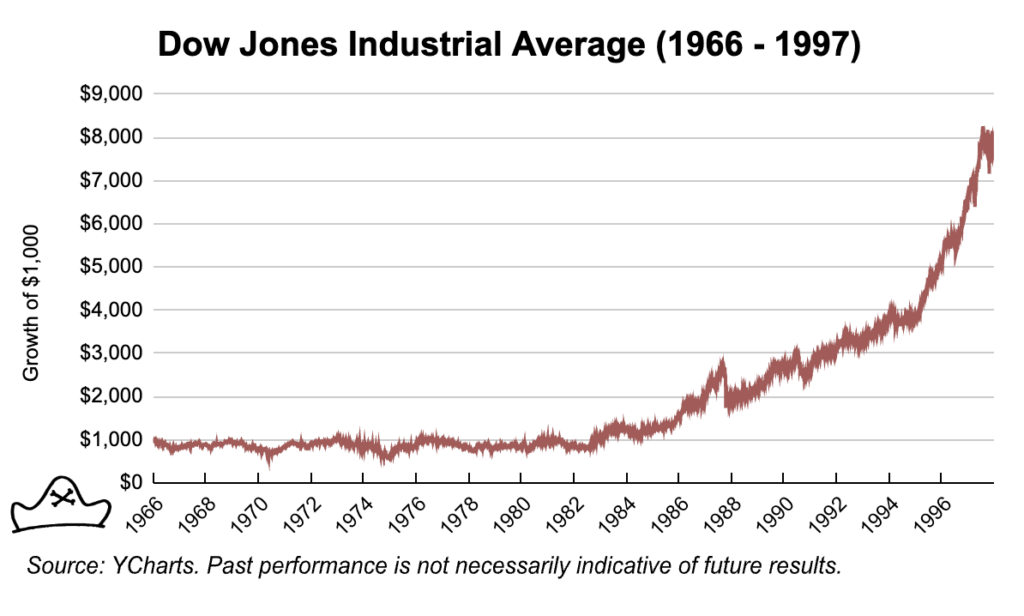
From 1966 to 1997 the Dow Index grew about 715% – an 8% average annual return.
However, those returns varied greatly over time. From 1966 through 1982 there are essentially no returns. $1,000 invested into the Dow Index at the beginning of 1966 was only worth about $1,080 by the end of 1982. Then, from 1982 through 1997 the Dow grew at about 15% per year taking the index from 875 to almost 8000.
Even though the average return was 8% over that period, the implications for an investor vary dramatically based on what order the returns come in.
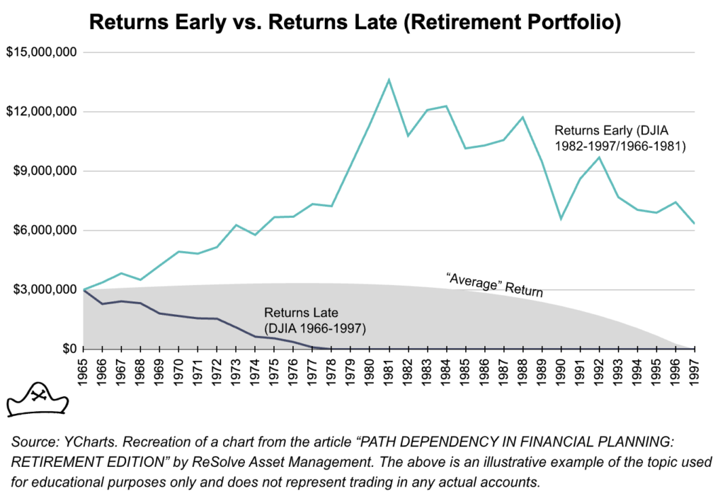
Consider a couple, Nick and Nancy, that has accumulated $3,000,000 in savings. They are ready to retire at age 63 and expect to draw $180,000 per year with that amount increasing 3% each year to account for inflation.4
If they experience the strong return period (1982-1997) first and the poor return period last (light blue line) then they will have more than enough funds to last through their retirement. Their wealth will increase even as they are withdrawing funds for the first decade or so leaving them plenty to draw down on in their later years.
However, if they get the returns in the order they actually happened, with a long flat period for the first 15 years, they go broke at age 76 (dark blue line).
Time matters. If big positive returns come early, Nick and Nancy are in great shape. If they come late, they are ruined. While the problem is most obvious in the case of retirement, anyone with outflows is subject to much the same dynamic. This could be someone who needed to use their savings in 1981 to buy a house, pay for their kids’ college education or start the business they’ve been thinking about for many years.
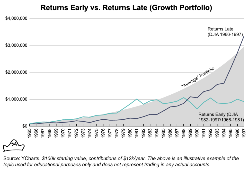
Now take someone on the other end of their career. Consider a 34 year old starting with $100,000 in savings and adding $1,000 per month to their savings account. If they get the good returns early (when they have relatively little savings) and the flat returns late then they finish with less than $1,000,000 ($913,815) at age 65 when they are ready to retire.
Conversely, if the flat returns come early and good returns come later when they have more capital to compound, they arrive at age 65 with $3,355,768 in savings. Achieving the smoother average return of 8% arrives at a similar figure of $2,955,960.
Using the popular 4% safe withdrawal rate, this is a difference between an annual expense budget of $36,552.60 (returns early) and $134,230.72 (returns late). There’s a big quality of life difference between $36,000 and $134,000 a year.
The difference between these two has nothing to do with how hard working or diligent in saving one was versus the other. It’s merely luck of when you were born and the path of returns over that period.
This is particularly worth keeping in mind for millennials and Gen X crowd that have experienced very strong post-2008 gains in equity markets.
A long decade or multi-decade flat period of equity returns could be extremely challenging for the mid-career equity focused investor, analogous to the investor getting the strong period of returns early and a weak period of returns late.
You do not necessarily get the average returns of the market.
You can drown in a river that is 2ft deep on average and you can go broke using a 4% withdrawal rate on a portfolio that has 8% average returns. If you have any inflows or outflows to your investment portfolio, you do not get the average returns of the market.
While we see most investors tend to evaluate investments based on their expected value, we believe it would be more prudent to think about their expected path.
We believe that the inclusion of defensive strategies that can do well in periods where equities struggle such as trend following and long volatility can help to increase the odds of a ‘good enough’ performance and improve long-term compounding.
Arguably risk-adjusted EV or risk-adjusted returns is something like Stage 2.5 as it is a significant improvement on merely thinking in terms of expected value.
Taylor has spent the last decade researching, consulting and speaking about how individuals and institutions can be more resilient and, if possible, antifragile. His research has been featured in dozens of media outlets including NBC, Inc, and The Financial Times. Connect with Taylor on Twitter @TaylorPearsonMe
Expected value (EV) is a popular and often cited concept among investors. However, it’s a bit of a misnomer and has a few serious limitations. To briefly recap, expected value is a calculation made by multiplying the probability of something happening by the magnitude of the outcome. Let’s say you give me a bet on a fair die. The die has 6 sides so each side should show up 16.6% of the time – that’s 6 to 1 odds. Now let’s say I offer you
“Stocks for the Long Run” is the mantra of many investors today. The U.S. stock market’s stellar performance, especially post 2008, and its rarity of long-term losses have become something of a gospel. Renowned experts like Eugene Fama and Ken French support this belief, estimating high probability of substantial gains over extended horizons. Indeed, the U.S. stock market was the strongest performing market in the 20th century. As Stocks for the Long Run author Jeremy Siegel noted: “… U.S. stocks have been the best long-term investment
We are excited to introduce a new addition to our suite of investment strategies – The Defense Strategy. It combines Mutiny Fund’s Volatility Strategy and Commodity Trend Strategy. The Volatility Strategy is designed to act as a so-called ‘black swan’ investment, achieving asymmetric gains in times of high volatility or tail risk (e.g. March 2020). The Commodity Trend Strategy is designed to profit during inflationary periods (e.g. 2022) as well as during extended ‘crisis periods’ for stocks and bonds (e.g. 2008). In combining these two
We use cookies to ensure that we give you the best experience on our website. If you continue to use this site we will assume that you are happy with it.
 This is an attractive bet: You are risking $1 and your expected payoff is $1.66.
Expected value is an important concept to understand that has broad applications across your life. Whether you are making an investment, career decision, or business decision, expected value is a valuable and important lens for thinking about it. 1
In my experience, the vast majority of investors use expected value as the primary model for thinking about an investment. When evaluating a new investment opportunity, they tend to try and determine the expected value of an investment and how it compares with other things they could invest in and to invest in the things which seem to have the highest expected value.
Most investing discussions are discussions around the EV (or risk-adjusted EV2
) of different assets or strategies.
Generally, a good understanding of expected value and some common sense will get you pretty far, but it’s important to understand the limitations of thinking strictly in these terms. I call these the Four Horsemen of Expected Value.
This is an attractive bet: You are risking $1 and your expected payoff is $1.66.
Expected value is an important concept to understand that has broad applications across your life. Whether you are making an investment, career decision, or business decision, expected value is a valuable and important lens for thinking about it. 1
In my experience, the vast majority of investors use expected value as the primary model for thinking about an investment. When evaluating a new investment opportunity, they tend to try and determine the expected value of an investment and how it compares with other things they could invest in and to invest in the things which seem to have the highest expected value.
Most investing discussions are discussions around the EV (or risk-adjusted EV2
) of different assets or strategies.
Generally, a good understanding of expected value and some common sense will get you pretty far, but it’s important to understand the limitations of thinking strictly in these terms. I call these the Four Horsemen of Expected Value.